
Content
March 4, 2026
Author: T. Jake Smith
The spread between wholesale beef prices and farmgate cattle prices has received considerable attention in recent years. The interest in this price spread has been driven by its trajectory. As shown in Figure 1, the farm-to-wholesale beef price spread remained relatively stable from 2000–2015. It increased notably from 2015–2019, spiked dramatically during 2020 and 2021, and decreased after 2021, finally returning to near pre-2015 levels by 2025.
Figure 1. Yearly Average Farm-to-Wholesale Beef Price Spread, 2000–2025

Note: Data from USDA-ERS Meat Price Spreads, available at https://www.ers.usda.gov/data-products/meat-price-spreads.
The sustained elevated price spread after 2015 generated intense interest in understanding the key drivers of the spread. Potential explanations have included beef packing firms’ ownership of multiple plants and the use of alternative marketing arrangements in the industry, but recent research suggests that the most important determinant of the price spread appears to be the capacity constraints of the beef packers.
How Capacity Constraints Drive the Price Spread
Every beef packing plant has a nominal slaughter capacity. This figure is usually given in units of head per day, but thinking about a plant’s operations and capacity constraints over the course of a week may be more enlightening. Plants typically operate Monday through Friday, with Saturday acting as a “shock absorber” when more processing is needed. We can think of a plant’s nominal weekly capacity, then, as being 5 times its nominal daily capacity. When the plant is operating below that capacity, its marginal processing cost—the cost of the labor, energy, and other inputs needed to transform the cattle into boxed beef—is relatively constant. The plant can exceed its nominal weekly capacity, but only with increasing marginal processing costs. That is, when it runs a Saturday shift (or pushes past its nominal daily capacity on a weekday), the plant faces higher per-unit costs due to factors like overtime pay for workers, forgone maintenance, and lower productivity.
The core ideas here—that processing costs are relatively constant below plants’ nominal capacities, and that nominal capacities can be exceeded but only with increasing marginal costs—can explain a lot about the farm-to-wholesale beef price spread. To see this, consider the simple model of beef and cattle supply and demand in Figure 2.[1] Consumers have a demand for beef represented by the demand curve DBeef. The demand curve shows the consumers’ marginal value for a given quantity of beef, and therefore the price at which that quantity can be sold. Packers’ willingness to pay for cattle comes from what they can earn selling beef to consumers, minus what it costs them to process the cattle into beef. This generates packers’ derived demand for cattle, DCattle.
Figure 2. Simple Model of Beef and Cattle Supply and Demand
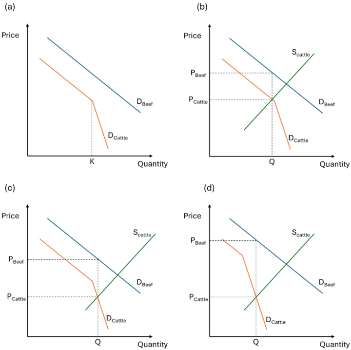
Note: Panel (a) shows the determinants of packers’ demand for cattle: consumers’ demand for beef and the industry capacity K. Panel (b) depicts an initial equilibrium where the industry is just below capacity. Panel (c) shows the equilibrium when the supply of cattle increases. Panel (d) shows the equilibrium when the effective industry capacity drops significantly, as during the COVID-19 pandemic.
Panel (a) in Figure 2 shows how capacity constraints impact packers’ demand for cattle. When the industry is operating below its capacity (labeled K), packers’ processing costs are constant, and their derived demand for cattle closely tracks consumers’ demand for beef. As the industry exceeds capacity, though, marginal processing costs increase, and packers’ willingness to pay for cattle declines more steeply than consumers’ willingness to pay for beef.
Panels (b), (c), and (d) in Figure 2 add cattle supply to the model to demonstrate how the forces of supply and demand shape the spread between beef and cattle prices. Panel (b) depicts an initial equilibrium where the industry is operating just below capacity. The quantity of cattle packers buy from producers, Q, and the cattle price, PCattle, are determined by the point where the cattle supply curve crosses the packers’ cattle demand curve. Packers process that quantity into beef and sell it at a price determined by consumers’ value for the beef, PBeef. The price spread is the vertical distance between PBeef and PCattle.
Panel (c) shows how the equilibrium changes when supply increases. The cattle supply curve now crosses the steeper portion of the packers’ cattle demand curve, leading to a higher spread between the beef price and the cattle price at the equilibrium quantity.
Finally, panel (d) illustrates the impact of a significant disruption to processing capacity, such as major plants shutting down during the COVID-19 pandemic. Such a disruption decreases the effective capacity of the industry, moving the “kink” in packers’ cattle demand curve to the left. Now, even with an unchanged cattle supply curve and consumer beef demand curve, the equilibrium changes dramatically. As the quantity supplied and the price of cattle decrease, the price of beef rises, and the price spread increases significantly.
Insights from the Model
This simple model of supply, demand, and capacity constraints in the beef packing industry has surprisingly impressive explanatory power. This can be seen in Figure 3, which shows monthly cattle slaughter volumes and farm-to-wholesale beef price spreads over 2016–2025. During this period, nominal industry capacity remained relatively constant, with few permanent plant openings and closings. The rising price spread from 2016–2019 corresponded with an upward trend in slaughter volumes, which we can think of as a gradual shift from panel (b) to panel (c) in Figure 2.
During much of 2020 and 2021, the effective capacity of the packing industry was severely disrupted by temporary plant closures caused by the COVID-19 pandemic and a cyberattack on JBS. We can understand these disruptions through the lens of panel (d) in Figure 2. In 2020, slaughter volumes decreased while the price spread widened significantly, exactly as in panel (d). In 2021, slaughter volumes remained at higher levels while the price spread skyrocketed even higher, which could be represented by the equilibrium in panel (d) with the cattle supply curve shifted to the right.
Finally, as the market returned to its normal capacity in 2022, we see a downward trend in both slaughter volumes and the price spread, which would correspond to a gradual shift from panel (c) back to panel (b) in Figure 2. Note that throughout 2025, slaughter volumes continued to decrease while the price spread remained relatively constant. This is precisely what the model would predict: once the equilibrium quantity drops below industry capacity, further decreases in supply will impact beef and cattle price levels, but not the spread between the two prices.
Figure 3. Monthly Industry Cattle Slaughter Volume and Farm-to-Wholesale Beef Price Spread, 2016–2025
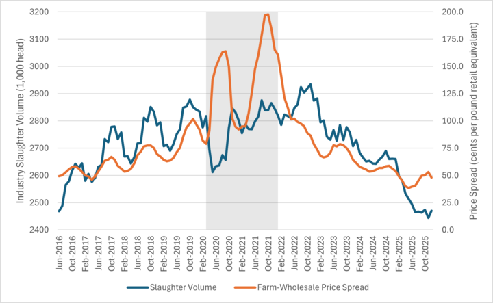
Note: Slaughter data from USDA-ERS Meat Statistics, https://www.ers.usda.gov/data-products/livestock-and-meat-domestic-data. Price spread data from USDA-ERS Meat Price Spreads, https://www.ers.usda.gov/data-products/meat-price-spreads. The figure shows the 6-month moving average of both data series. The shaded area covers March 2020–December 2021, when major disruptions to the packing industry’s effective capacity (including COVID-19 and a cyberattack on JBS) occurred.
Conclusion
The elevated levels of the farm-to-wholesale beef price spread since 2015 and the dramatic spike in the spread during 2020–2021 have generated intense interest in this measure by cattle producers, policymakers, and agricultural economists. The simple model presented here, in which beef packers’ demand for cattle is determined from the combination of consumers’ beef demand and packers’ processing costs in the presence of capacity constraints, can help us understand the supply and demand factors that drive the price spread. While this model assumes away some complicating factors, like industry concentration and the use of alternative marketing arrangements, that also influence the price spread, research shows that capacity constraints are the primary determinant. For further information on the interaction between market structure, alternative marketing arrangements, capacity constraints, and price spreads in the beef packing industry, see Moschini and Smith (2025).
Further reading:
Moschini, G. and T.J. Smith. 2025. “Spatial price competition and buyer power in the U.S. beef packing industry.” American Journal of Agricultural Economics. https://doi.org/10.1111/ajae.70003
Author Contact:
T. Jake Smith
Assistant Professor
Department of Agricultural Economics
University of Nebraska – Lincoln
tsmith125@unl.edu
[1] This model makes many simplifying assumptions. These assumptions include: Cattle is processed into beef in fixed proportions; Cattle and beef are measured in such a way that 1 unit of cattle translates into 1 unit of beef; Beef packers all have the same cost structure; and beef packers set beef and cattle prices competitively (i.e., marginal cost/marginal value pricing). While we know these assumptions don’t all hold in the real world, they allow us to focus squarely on how capacity constraints drive price spreads.